How Baseline Works

At its core, every Baseline token is managed by the Baseline Market Maker (BMM), a novel AMM that allocates liquidity more intelligently, facilitating better price discovery and creating more efficient token markets.

Why It Matters

Most markets today use central limit order books to allocate liquidity. This approach requires every project to negotiate deals to bootstrap liquidity, and have professional market makers to actively manage quotes. In a world where most assets are issued digitally at an accelerating pace, this is no longer a viable solution.

Algorithmic Market Makers (AMMs) solve this by replacing active management with a bonding curve, a mathematical formula that quotes prices automatically using pooled liquidity. This approach, however, treats liquidity separate from the token, creating problems:

Liquidity mismatch: Pools quote without knowing float, causing either low-float pumps (too much liquidity) or death spirals (too little liquidity)
Value leakage: Most popular AMMs deploy liquidity even when they should protect reserves
Death spirals: Without awareness of circulating supply, the AMM is unable to backstop negative market reflexivity, causing tokens to trend to zero.

The Baseline Market Maker (BMM) enables Baseline tokens to move beyond limitations of traditional markets to programmable markets that actively grow the economies they represent.

How It Works

Token-owned liquidity tracks circulating supply ( $c$ ), pool inventory ( $x$ ) and pool reserves ( $y$ ) in a single smart contract. Pool reserves are split into backing reserves and buffer reserves:

y = y_{backing} + y_{buffer}

Backing reserves guarantee every circulating token can be redeemed at the floor price
Buffer reserves enable price discovery above the floor

Baseline Value (BLV)

BLV is the guaranteed floor price that determines how backing reserves are allocated:

P_{blv} = \frac{y_{backing}}{c}

Equivalently:

y_{backing} = P_{blv} \cdot c

This invariant is enforced programmatically at the smart contract level, ensuring every circulating token can be redeemed at, or above, the floor price. The BLV can never decrease but, through the token's market making operations, the BLV can increase over time.

The Buffer Invariant

Buffer reserves follow a power-law curve based on inventory ratio:

y_{buffer}\cdot \left(\frac{x}{c}\right)^2 = K

The invariant maintains a constant K by adjusting buffer reserves based on the inventory ratio (x/c):

High circulation (x is small, c is large): Inventory ratio is low, so buffer reserves are large. The pool deploys deep liquidity to facilitate price discovery as tokens trade actively.
Low circulation (x is large, c is small): Inventory ratio is high, so buffer reserves shrink. The pool withdraws liquidity as it absorbs supply, transitioning from price discovery to price protection at the floor.

Liquidity Efficiency

BMM allocates liquidity based on two ratios that work together.

Inventory Ratio measures pool inventory relative to circulating supply:

R_{inventory} = \frac{x}{c}

Buffer Ratio measures buffer reserves relative to total reserves in the pool:

R_{buffer} = \frac{y_{buffer}}{y}

Traditional AMMs ignore these relationships, which causes problems in extreme states. BMM, on the other hand, maintains a bounded liquidity efficiency:

L_{efficiency} = R_{buffer} \times R_{inventory}

This ensures liquidity allocation stays efficient across all circulation states. As inventory ratio increases, buffer ratio decreases proportionally, preventing the system from over-allocating liquidity when it should be protecting the floor.

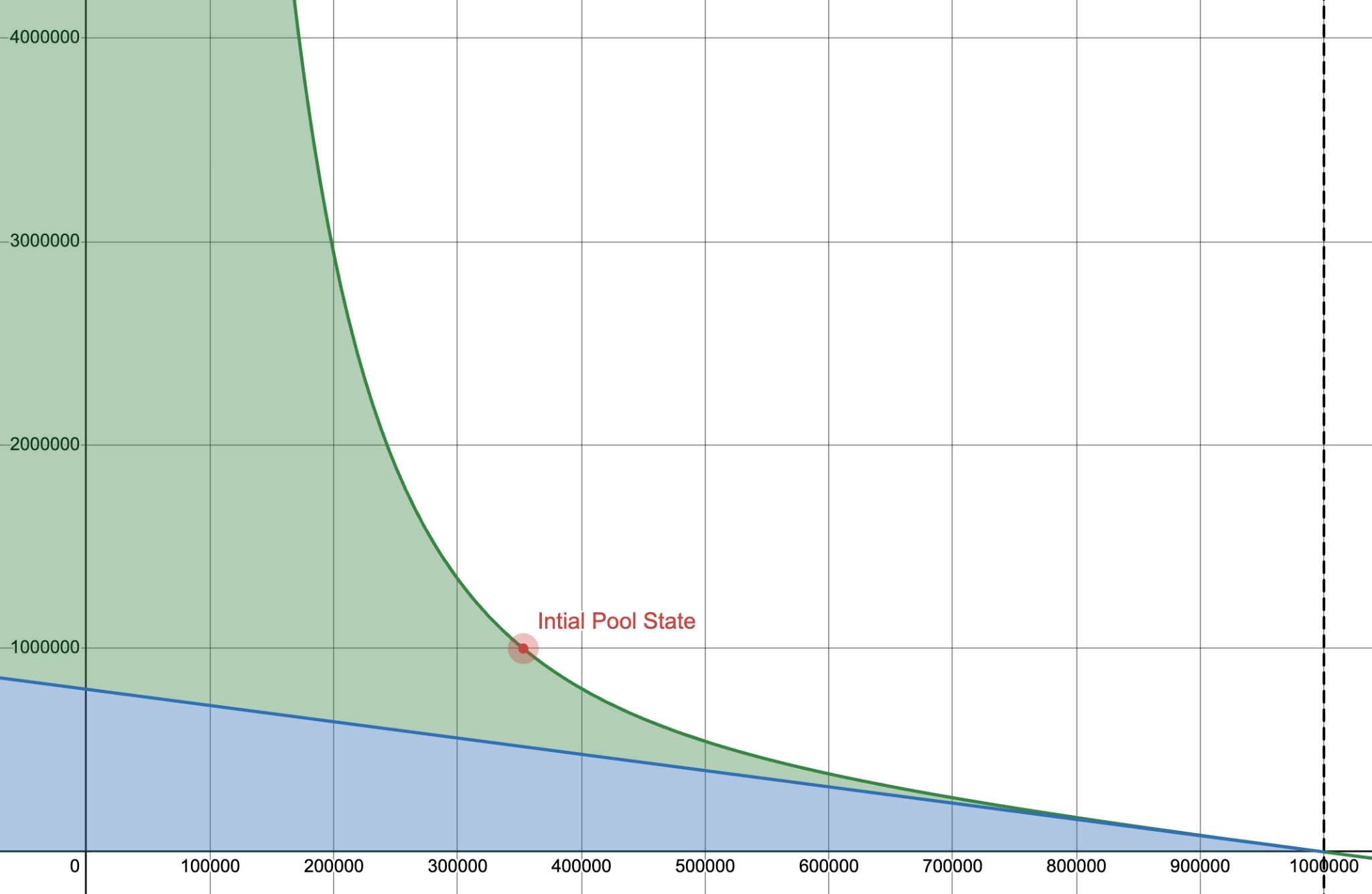
Example

The chart below shows pool inventory on the x-axis and total reserves on the y-axis. The blue area represents backing reserves required to buyback all circulating supply at the floor. The green area represents buffer reserves available for price discovery.

Reserves Curve showing backing and buffer reserves

Baseline vs Traditional AMMs

Traditional constant-product AMMs (xy=k) have a fundamental limitation: they deploy all reserves for trading with no floor protection. Using the definitions above, in xyk systems, we have:

$y_{backing} = 0$ (no concept of backing reserves)
$y_{buffer} = y$ (all reserves used for price discovery)
$P_{blv} = 0$ (no floor price, tokens can go to zero)
$L_{efficiency} \rightarrow \infty$ as $c \rightarrow 0$

This creates several problems:

Liquidity mismatch: Pools quote without knowing float, causing either low-float pumps (too much liquidity) or death spirals (too little liquidity)
Value leakage: Reserves get extracted even when the system should be protecting them
No defensive mechanism: Traditional AMMs don't transition from price discovery to price protection

BMM solves this by being circulation-aware and splitting reserves into backing and buffer. As circulation collapses, BMM automatically withdraws buffer liquidity and transitions to price protection, preventing the distortions that plague traditional AMMs.

Key Concepts

Baseline Value (BLV): The guaranteed floor price mechanism
Baseline Market Maker (BMM): The circulating-supply-aware AMM
Fees: How fees grow the floor price

Points Program Baseline Value (BLV)